with Sahil Chhabria, Junior Analyst Aroha Capital
This blog is an attempt to conduct an analysis of the excess return of some of the Flexicap Mutual Funds in India. Thereon we have proceeded to conduct an attribution analysis of the Timing and Selection components of these excess returns.
Background
We are proponents of passive investing with a focus on low cost, low tax drag, simplicity and genuine diversification. On the occasion we have given a nod to actively managed funds where we see a manager who has generated excess returns over the benchmark at risks comparable to the benchmark. We have discussed in the past the key elements of passive funds which are Tracking Error and Expense Ratio. Active funds on the other hand are largely measured on their ability to consistently generate excess return over the benchmark. The sources of excess returns for an active fund can be either:
- Having a more risky portfolio (or)
- Superior Timing of Asset Class /SectorAllocation (or)
- Superior Security Selection within each Asset Class/Sector
Sources of our data include:
- Daily NAV (Nett Asset Values) of top 7 Flexi Cap Funds by AUM from 30-Nov-2015 to 31-Aug-2025 taken from the AMFI (Association of Mutual Funds of India) website.
- Fund Fact Sheets: Monthly asset allocation to Core Indian Equity, US Equity, and Cash taken from the respective mutual fund websites
Benchmark Composition:
- Nifty-50 TRI: 100%
- S&P 500 in INR: 0%
- SBI Liquid Fund: 0%
The rationale is that Flexicap Funds in India are largely benchmarked to the Nifty-50 TRI. However many take significant exposure to Cash and at-least one of them takes a non- trivial exposure to US Equity. We used SBI Liquid Fund as our Benchmark for Cash – as we were unable to get access to a suitable index for cash.
5-Year Rolling Excess Return vs Nifty-50 TRI:
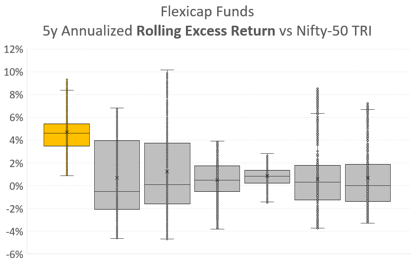
This chart compares each fund’s performance relative to the benchmark.
- Highlighted Fund: The highlighted fund has a Median excess rolling return of ~5% with a narrow Interquartile Range (IQR). In-fact there is no period where the fund has generated negative excess return over a rolling 5 year period from Nov-2015. This indicates a genuine ability to consistently outperform the benchmark.
- Peers: Mixed results. Some funds show negative medians and wide IQRs. In-fact every other fund has excess return spanning both positive and negative ranges indicating an inability to consistently deliver excess return.
Insight: The highlighted fund is a clear outperformer, combining high median returns with stability.
We now turn our attention into understanding the components of the excess returns shown in the above chart. The Brinson Model provides an Attribution Framework that decomposes excess return into:
- Selection effect: Security-level outperformance within asset classes
- Timing effect: Tactical allocation between asset classes
Brinson model:
Developed by Gary Brinson and colleagues in the 1980s, the Brinson model is widely used in institutional portfolio analysis. It compares a portfolio’s returns to a benchmark by examining:
- Allocation/Timing Effect: Did the manager overweight or underweight asset classes that performed well?
- Selection Effect: Did the manager pick better-performing securities within each asset class/sector?
- Interaction Effect (optional): Did the manager simultaneously allocate well and select well in the same as
The Brinson Model discusses 4 quadrants:
| Quadrant | Description | Comments |
| I | Benchmark | Benchmark Weights and Benchmark Returns |
| II | Benchmark & Timing | Portfolio Weights and Benchmark Returns |
| III | Benchmark & Selection | Benchmark Weights and Portfolio Returns |
| IV | Portfolio | Portfolio Weights and Portfolio Returns |
Amongst the 4 quadrants above, all of them are calculable, except quadrant III – wherein we do not have access to the Asset Class/Sector Returns of each Asset Class/Sector within the fund. The 4 quadrants above can be used to decompose the returns into Timing, Selection and Interaction as follows:
| Effect | Formula |
| Timing | II-I |
| Selection | III-I |
| Interaction | IV-III-II+I |
| Total Excess Return | IV-I |
Since quadrant III is incalculable, we make a simplifying assumption that Interaction Effect = 0. If we make this assumption, and rearrange the Interaction Formula we get:
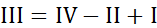
With the simplifying assumption that the Interaction Effect is zero, we now have values for all 4 quadrant and are in a position to calculate the Timing and Selection components of the Excess returns.
We went back about 10 years (since Nov 2015) for the selected 7 Flexicap funds and extracted from their fund fact sheets exposures to Core Indian Equity, US Equity and Cash on a monthly basis. We then calculated quadrants I, II, III and IV on a monthly basis and used these numbers to decompose returns into Selection and Timing effects again on a monthly basis. We converted these monthly returns into 5 year rolling returns and then tabulated the data in the form of box and whisker plots which we will discuss below. Do note that the charts below are data extracted for 5 year rolling returns with a monthly resolution (as against a daily resolution used for Chart 1 above).
Chart 2: Attribution from Timing
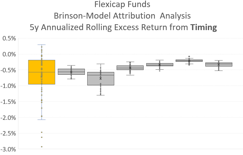
This chart isolates the impact of tactical allocation (Timing) decisions.
- Highlighted Fund:
- Median timing return: ~-0.5%, similar to peers
- IQR: wider spread, suggesting allocation has wider ranges
- Peers:
- Most show similar negative timing effects (~0% to -2%) though with tighter IQR bands suggesting narrower allocation ranges.
Insight: Timing generally detracted from performance. The highlighted fund is similar to other funds on an average though IQR is wider indicating wider allocation ranges.
Chart 3: Attribution from Selection
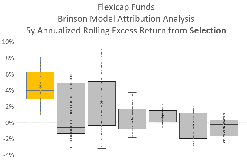
This chart evaluates stock-picking skill within asset classes.
- Highlighted Fund:
- Median selection alpha: ~5%, highest among all funds
- IQR: Narrow and no negative values, indicating consistent selection skill
- Outliers: None, reinforcing reliability
- Peers:
- Mostly positive medians but wider IQRs
- IQRs span both positive and negative ranges indicating inconsistent selection skill
Insight: Selection on an average contributed to performance for all funds with the highlighted fund significantly superior to its peers. The highlighted fund was significantly superior in that it had a very tight IQR and there were no 5 year rolling periods over which its Selection excess returns were negative.
Conclusions:
- The highlighted fund stands out for its consistent outperformance particularly its strong selection outperformance. It also seems that the highlighted fund has taken more extreme allocation/timing decisions which have detracted from its performance with more variability – however this is more than compensated with the manager’s superior stock selection skills.
- Other Flexicap funds, suffered in their inability to consistently achieve positive stock selection capability (although on an average they were positive).
- Selection is the primary driver of excess return across funds, while timing generally detracted.
Disclaimer
We suspect our assumption of Interaction Effect = 0, may not be entirely correct. Our first pass analysis indicates that the timing and selection effects as calculated above are mildly correlated – indicating that there is at-least some interaction effect at play. Unfortunately, in the absence of public information on the returns within asset classes/sectors of each of the funds we are not in a position to assess the same.